

Types of Algorithms and Their Applications
This article is part two of “What Algorithms Are and What You Should Know About Them” by RDI Communications Specialist Martti Asikainen and senior reacher Janne Kauttonen. In this article we dive into the more technical concepts of algorithms. You can find the first part of the article here.

Martti Asikainen & Dr. Janne Kauttonen, 20.3.2025
Algorithms are a central part of modern technology. They are like precise instructions that perform defined operations step by step. At their simplest, an algorithm can arrange numbers in series, while at their most complex, they can direct not only the operation of artificial intelligence but also influence the flow of information we receive in the form of recommended content. In this article, we take a deeper dive into the different types of algorithms and their applications. We begin with search algorithms, which are among the simplest yet most versatile algorithms, found in nearly every program that processes information.
Search algorithms are typically divided into linear search and binary search. Linear search systematically scans each element in an array until the target value is found (Cormen et al., 2009). In contrast, binary search operates similarly to looking up a word in a dictionary—it starts in the middle, then directs the search toward either the beginning or the end, repeatedly halving the search area. However, binary search requires that the dataset be sorted in either ascending or descending order (Knuth, 1998; Grossman & Frieder, 2004). This means the data must first be organized, but once sorted, binary search provides a much faster lookup compared to linear search.
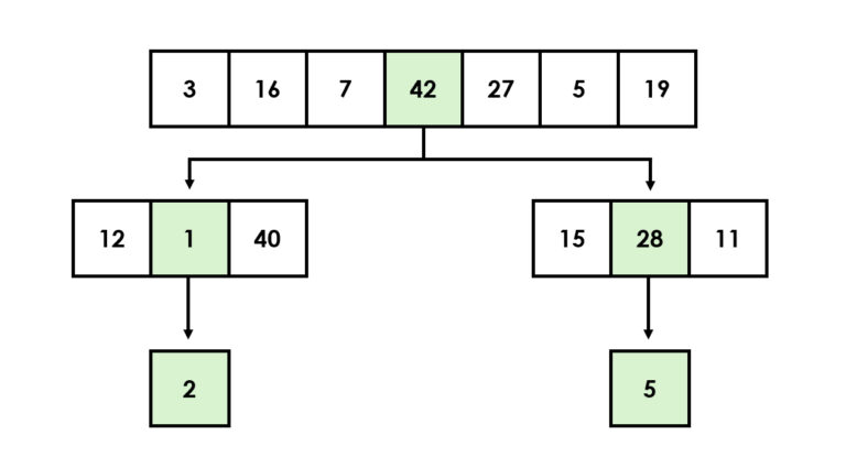
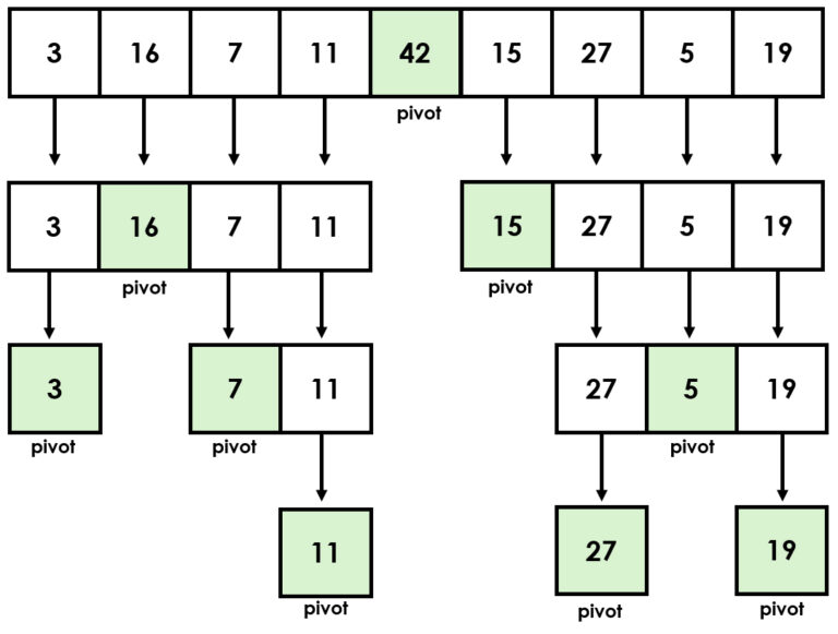
Sorting algorithms fight against chaos and create order by rearranging data structures using a comparative operator. One of the most well-known sorting algorithms is quicksort, which utilizes the divide and conquer principle by dividing the data set into smaller parts and processing them recursively (Hoare, 1962).
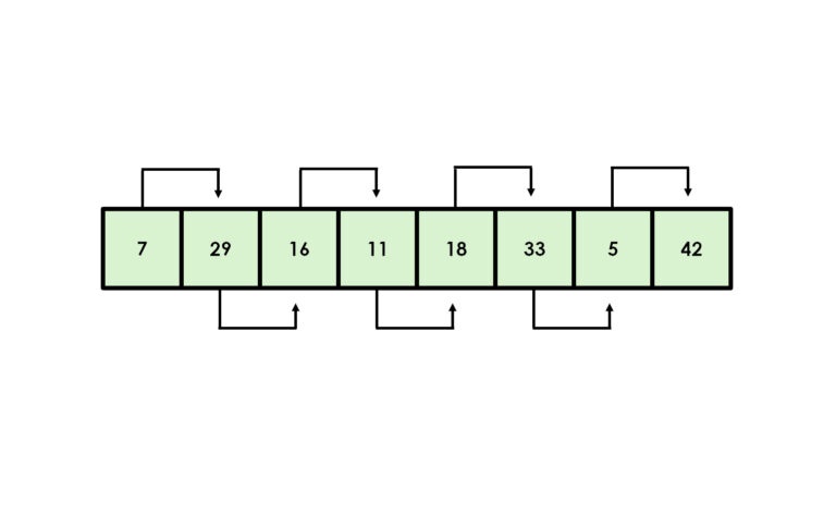
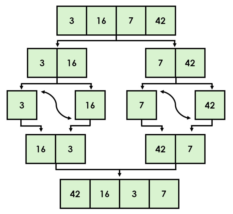
Another efficient sorting algorithm is merge sort, which combines subsets in order (Cormen et al. 2009). Simpler algorithms, such as bubble sort and selection sort, can also be useful. However, according to experts, these are mainly suitable for educational purposes and visual presentations (Sedgewick & Wayne, 2011).
From Merge Sort to Clustering
Like the previously discussed binary search and quicksort, merge sort is also a recursive algorithm that, similar to a Russian matryoshka doll, contains smaller versions of itself. Recursions always have two parts: the base case, which is the situation where the answer is known, and the recursive case, which is solved by breaking it down. For this reason, they are also called divide and conquer algorithms, tamers of large problems that break a big problem into smaller pieces and solve them until the entire task is complete.
Another practical example could be a situation where your files are in disarray. Completely jumbled, and you would like to organize them using an algorithm. A recursive algorithm would first open the main folder, go to the first subfolder and then to that subfolder’s subfolder to organize it according to the method defined in the base condition. From the lowest folder, it would always move upwards climbing the folder tree, using the same principle, until all files were in order, after which it would move to the next folder. This principle is utilized, for example, in file management and in the structures of websites.
One of the significant advantages of merge sort is its ability to operate efficiently in linked lists without the need for additional memory space. However, its use is not limited to simple sorting. It can also be utilized to calculate inversions in a list, which is useful for example in analyzing data structures or evaluating the complexity of sorting operations.
Furthermore, merge sort is an excellent choice for external sorting, where data volumes are so large that they cannot fit into a computer’s memory all at once. It is especially valuable, however, in situations where data stability matters. In stable sorting, elements of equal value retain their original relative order even after sorting, which improves the readability and usability of the data.
Imagine, for example, a table where people are first sorted by name and then you want to sort them by age groups. With merge sort, people of the same age still remain in alphabetical order.
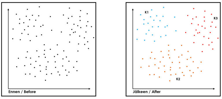
When discussing segmentation, one cannot bypass k-means clustering, which is one of the most common and simplest unsupervised machine learning clustering algorithms. It is classified as an unsupervised machine learning method. Its purpose is to divide a dataset into a predetermined k number of groups or clusters, where observations are as similar as possible to each other (e.g., MacQueen 1967). It can be used, for example, for image recognition, customer segmentation based on purchasing behavior, demographic information, or online behavior.
Other uses include document classification, creating pricing strategies (optimal price levels for different segments), identifying anomalies or unusual events (banks, financial sector, research), personnel analytics (employee profiles and competency needs), inventory management (grouping products based on sales, seasonal variation, or inventory turnover), recommendation systems (similar customers or products), and market analyses (competing companies or market areas).
A grocery store, on the other hand, could apply clustering for example by clustering products according to consumer purchasing behavior, after which the products in the store are arranged based on the clustering. As limitations of k-means clustering, it can be stated that they work best with spherical clusters and the results depend on the selection of the initial centroids. Additionally, it is sensitive to outliers and its operation requires determining k, the number of clusters, in advance.
Basics of Graph Algorithms
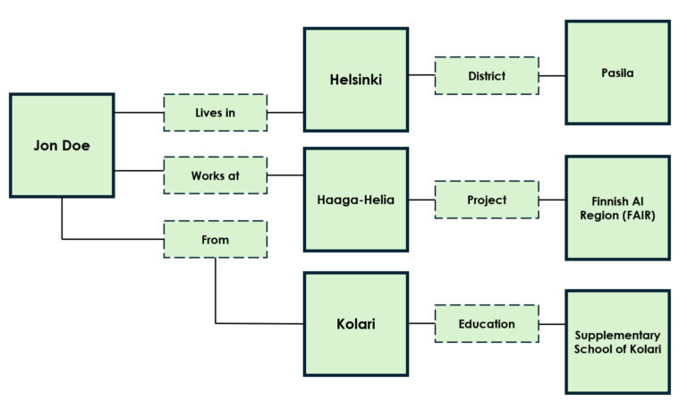
When discussing file management, it is also essential to understand the basics of graph databases, as graphs provide a natural way to represent networked information. Graph databases organize information according to the graph data model, where nodes and their connections or edges appear as a clear data structure (Angles & Gutierrez 2018). This allows natural modeling of data instead of treating data points as separate from each other. Nodes and connections can have many different properties that contain additional information—each node or connection represents some other property in the database. A graph enables many operations that are laborious for a simple tabular data structure. For example, finding interconnected information is easy in a graph data model.
Today, many well-known companies swear by graph databases and algorithms due to their agility, scalability, and performance. Their suitability for networked data and ability to reveal complex, often hidden connections between different pieces of information can also be counted as advantages. This increases explanatory power, for example, in various analyses that require visualization capabilities. Other strengths include the flexibility of the database schema and the comprehensibility of the graph data model (e.g., Thitz 2023). The graph data model is particularly applied in social media, semantic web, and biology fields (Barceló et al. 2011).
Although algorithms based on graph databases might sound unfamiliar, you probably encounter them daily. Familiar applications such as Instagram, Facebook, and X use graph algorithms to connect users, their preferences, and map recommendations. Google’s original search engine was also based on a graph algorithm called PageRank. Graph algorithms are indeed a quite considerable alternative to traditional tables and relational database-based solutions.
Greedy Algorithms from Dijkstra to Prim
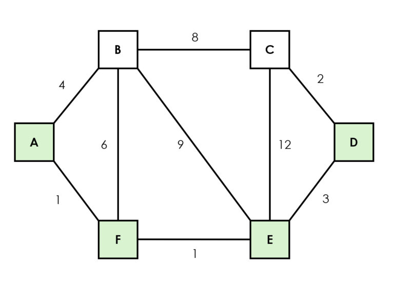
Path-finding algorithms are important in graph theory and absolutely necessary for handling networks. Dijkstra’s algorithm is one of the most used path-finding algorithms for finding the shortest path in a graph (e.g., Google Maps movement optimization), where all edge weights are non-negative (Dijkstra, 1959). Other path-finding algorithms include Prim, which builds a network by adding the shortest connections to new nodes, and Kruskal, which always selects the shortest possible connection such that the connection does not form a loop.
The A* algorithm is an extended version of Dijkstra’s algorithm and is used especially in games and navigation applications where the aim is to speed up finding the optimal route from a starting point (or node) to other points using heuristics, such as Euclidean metrics and Manhattan distance (Hart et al. 1968).
Dijkstra, A*, Prim, and Kruskal are sometimes also classified as so-called greedy algorithms, which also include algorithms such as activity selection problem, Huffman coding used for data compression, and the coin change greedy approach, where the algorithm would always give change with the largest possible units.
Greedy algorithms work like children in a candy store. They make what appears to be the best choice at each step based on the information available at that moment. They also have no backtracking, so they never reverse choices they’ve made, even if they prove to be poor for the overall solution, because they form the solution step by step. The main challenge of greedy algorithms is to find a suitable use case where the greedy strategy produces an optimal solution. The problem must be such that what currently appears to be the best choice also produces the best overall result. On the other hand, a greedy algorithm is quick and easy to calculate, so it can be a viable alternative in situations where the solution does not need to be optimal.
When discussing path-finding algorithms, it is also appropriate to mention the Bellman-Ford algorithm, which calculates the shortest distances for all nodes from one node and is used, for example, in optimizing economic costs, as well as the Floyd-Warshall algorithm, which is based on dynamic programming and is particularly utilized in business analysis. It calculates the shortest distances between all nodes. It is particularly suitable for dense graphs and situations where one wants to know the minimum cost between nodes.
Brute Force and Dynamic Programming
The brute force algorithm is useful for stress tests, but it is also used to crack passwords, login information, and encryption keys. The brute force algorithm is as persistent as a safe cracker who tries and listens to every different combination to open the door. It’s not very skilled, but rather a digital determined individual who relies on pure perseverance. At the same time, it is perhaps the simplest and most basic algorithm, and therefore quite inefficient in complex problems.
The operating principle of the brute force algorithm is simple. For example, if your phone were locked with a four-digit PIN code, and you wanted to open it using a brute force algorithm, the algorithm would go through every possible option between 0000-9999 (0001, 0002, 0003…) to open it. The algorithm can also be used for optimization and route-finding problems (e.g., the traveling salesman problem, TSP), where the shortest route between different destinations is sought.
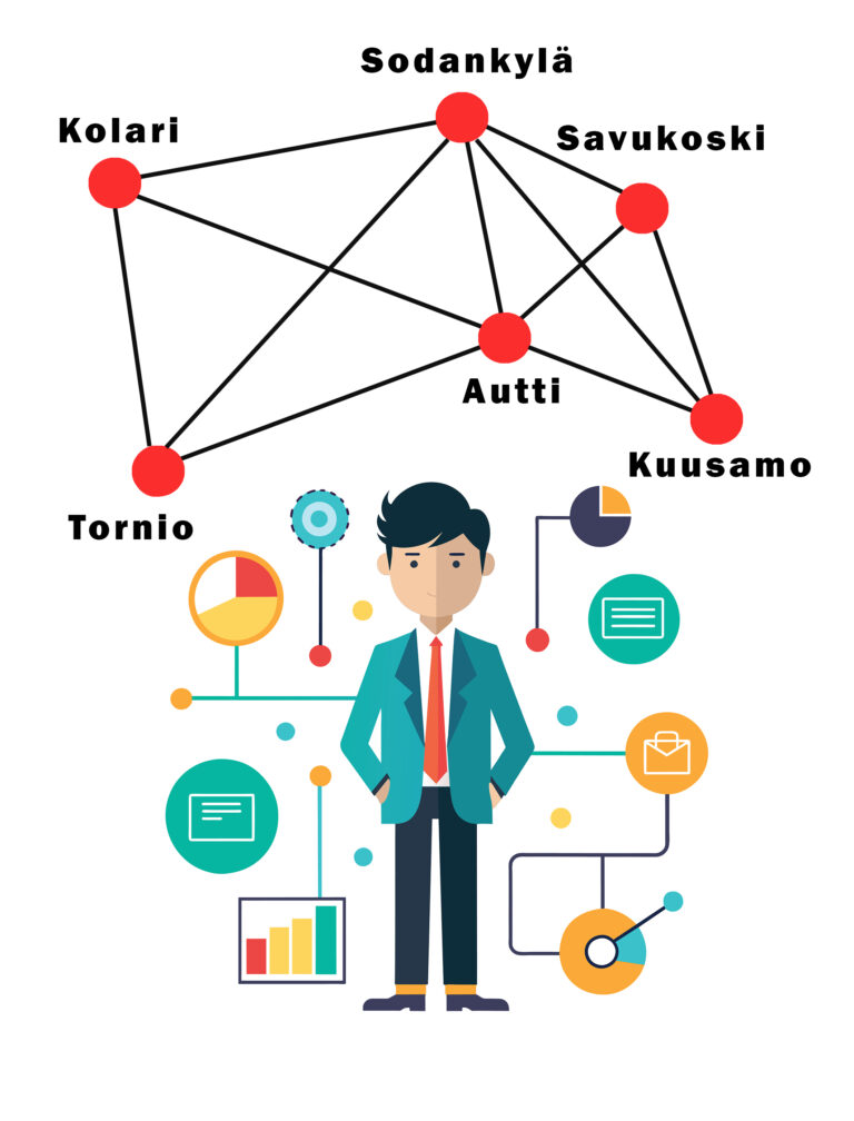
In the traveling salesman problem, the salesman knows the mutual distances between cities. The question is how can he calculate the fastest (shortest, cheapest) route for himself, where all nodes are visited only once, and finally return to the starting point. With a brute force algorithm, this happens by calculating the total number of routes, after which all possible routes are listed.
After this, the distance of each route is calculated, and finally, the shortest possible existing route is selected. If there are many cities (around 30), the problem becomes enormous, and even the computational power of the best supercomputer will be exhausted when using a brute force algorithm.
Dynamic programming is a method where complex problems are solved by dividing them into smaller parts and storing intermediate results so that the same calculations do not need to be repeated. They differ from traditional divide and conquer algorithms in that a dynamic programming algorithm divides the problem into overlapping parts and uses previously calculated results by storing them again, whereas divide and conquer algorithms divide the problem into independent parts, which it solves separately and combines the final result.
In other words, dynamic programming algorithms are like experienced puzzle builders who easily learn to recognize recurring patterns. They break down a complex problem into smaller parts and partially overlapping pieces, and when the solution to one piece has been found, they store the answer in their memory for later use. The solution is indeed most suitable for many classic data processing challenges, such as the knapsack problem, calculating Fibonacci numbers (where each number is the sum of the previous two: 1,1,2,3,5,8…), where the algorithm stores already calculated values (memoization/tabulation), and thus avoids unnecessary calculation (e.g., Bellman, 1957; Cameron 1994; Brualdi 2005).
The dynamic programming algorithm is used above all for optimization. It saves computation time and thus significantly improves efficiency. If the same problems were answered using a divide and conquer style and purely recursively, the calculation method would be quite inefficient because the same values are calculated multiple times. Other commonly known problems to which dynamic programming offers a solution are the longest common subsequence problem (LCS), Matrix Chain Multiplication, the Coin Change Problem, and the Edit Distance problem (e.g., Levenshtein distance).
Randomization and Feedback
In the disciplined world of programming and algorithm design, processes typically adhere to precise plans without room for surprises. Yet paradoxically, randomness and chance have emerged as essential components of numerous modern applications and computational methods. This apparent contradiction reveals one of computing’s most fascinating dimensions.
Randomized algorithms constitute their own distinctive category that harnesses unpredictability as an integral part of problem-solving. Rather than fitting neatly into traditional algorithm classifications, they represent a versatile design technique applicable across diverse algorithmic challenges. What makes these algorithms unique is their deliberate reliance on controlled randomness within their logic, strategically employed to reduce execution time and simplify complex problems. The quicksort algorithm exemplifies this approach—by selecting a random pivot point rather than a fixed value, it frequently achieves superior performance.
These randomized approaches fall into two principal categories. Monte Carlo algorithms may occasionally produce incorrect results with a calculable probability, accepting this trade-off for speed and simplicity. In contrast, Las Vegas algorithms guarantee correct results but operate with varying and unpredictable execution times. Both approaches find their niche in scenarios where determining an exact solution would prove prohibitively slow or complex, making a close approximation entirely acceptable.
The applications for such randomized methods span numerous fields including cryptography, numerical integration, optimization problems, and statistical data analysis. Randomization provides elegant solutions to practical challenges that lack a single optimal answer.
Consider the restaurant industry, where many establishments employ randomized algorithms during peak hours. Instead of processing orders strictly sequentially—which often creates bottlenecks for certain dishes—these systems randomly select the next order to prepare from those waiting longest, effectively reducing average wait times while maintaining consistent kitchen workflow

Complementing these randomized approaches are feedback algorithms, which belong to the category of iterative algorithms. They are typically part of dynamic systems or machine learning, where the results of previous executions are used as input in subsequent runs. In other words, they learn and adapt from the results of previous performances.
More specifically, feedback algorithms can be classified into control algorithms, where the system’s output is monitored and used to adjust future inputs; learning algorithms, which improve their performance based on the system’s previous results; and optimizing algorithms, which iteratively try to find the best possible solution using previous results.
Practical examples of feedback algorithm applications include the backpropagation algorithm in neural networks, PID controllers, and genetic algorithms. They differ from backtracking algorithms in that backtracking algorithms build solutions incrementally and retreat when they notice that the current path does not lead to the desired solution, whereas feedback algorithms learn from their mistakes.
This can be conceptualized by imagining a labyrinth from which we are trying to escape using an algorithm. A backtracking algorithm would systematically go through the entire labyrinth, and would always retreat when encountering a dead end, while a feedback algorithm could learn the structure of the labyrinth by heart based on its previous attempts and improve its performance after each attempt.
Both algorithms have their time and place. The systematic approach of backtracking algorithms, for example, is perfectly suited for solving complex puzzles and for the gaming industry. It is used to find solutions to Sudoku puzzles, AI-enhanced chess games, molecular modeling, and planning robot trajectories.
Feedback algorithms, on the other hand, have revolutionized the field of neural networks and made deep learning possible. Classic feedback problems include, for example, the Hamiltonian cycle, which passes through each point in a network exactly once (see the traveling salesman problem), as well as the rat-in-a-maze problem typical of IKEA department stores, where the goal is to find a way out when all corridors look the same.
What makes these algorithmic approaches so powerful is their reflection of natural processes. Just as evolution employs both random mutation and selective feedback to develop increasingly sophisticated organisms, these algorithms harness controlled randomness and systematic learning to solve problems that would otherwise remain intractable.
In embracing randomness, computer science has discovered not chaos, but a sophisticated tool for managing complexity in an uncertain world.
Summary and Conclusion
Now you have read our two part article “What Algorithms Are and What You Should Know About Them”. The technical exploration of algorithm types reveals the diverse computational methods powering modern technology. From fundamental search and sorting algorithms that organize data to specialized clustering techniques that segment customers, each serves a distinct purpose.
Graph algorithms enable complex relationship mapping while pathfinding algorithms optimize routes across networks. More advanced approaches like dynamic programming solve complex problems by storing intermediate results, while randomized and feedback algorithms introduce controlled variability and self-improvement mechanisms.
Together, these algorithmic approaches form the foundation of computational problem-solving across industries—from e-commerce recommendations to logistics optimization—demonstrating how mathematical principles translate into practical business advantages when correctly implemented.
For SMEs, the implementation of algorithms does not require large initial investments or profound technical knowledge. Many digital platforms and software already contain advanced algorithms that can be implemented without coding skills:
- Data collection and organization. The efficiency of algorithms depends on the quality and quantity of available data. Customer information, sales statistics, and product-specific information form a valuable foundation.
- Cloud-based analytics tools offer cost-effective solutions for SMEs. Microsoft Power BI, Google Analytics, and many industry-specific software include ready-made algorithms that can be implemented without significant IT investments.
- Agile experimentation and learning are key. Start small, for example, with the algorithmic analysis of one product group or market segment, and expand usage based on results.
In the future, algorithmic decision-making will only strengthen, and its importance for competitiveness will be further emphasized. For SMEs, it is of paramount importance to keep up with developments, as algorithms offer the opportunity to operate more nimbly and efficiently than competitors.
We also recommend contacting free services like the Finnish AI Region (FAIR), through which you can get advice and support in mapping and implementing algorithms as part of your business.
Contact us

Janne Kauttonen
Senior Researcher
+358 294471397
janne.kauttonen@haaga-helia.fi

Martti Asikainen
RDI Communications Specialist
+358 44 920 7374
martti.asikainen@haaga-helia.fi
References
Angles, R. & Gutierrez, C. (2018). An introduction to graph data management. In Fletcher, G., Hidders, J. & Larriba-Pey, J. L. (eds.), Graph Data Management, 1–32. Springer International. Cham.
Barceló, P., Libkin, L. & Reutter, J. (2011). Querying graph patterns. Proceedings of the Thirtieth ACM SIGMOD-SIGACT-SIGART Symposium on Principles of Database Systems, 199–210.
Bellman, R. (1957). Dynamic programming and stochastic control processes. Information and Control 1 (3), 228-239. Elsevier. Amsterdam.
Brualdi, R.A. (2005). Introductory Combinatorics. 5th edition. Pearson. London.
Cameron, P. (1994). Combinatorics: Topics, Techniques, Algorithms. Cambridge University Press. Cambridge.
Cormen, T. H., Leiserson, C. E., Rivest, R. L., & Stein, C. (2009). Introduction to Algorithms (3rd ed.). MIT Press. Cambridge.
Dijkstra, E. W. (1959). A note on two problems in connexion with graphs. Numerische Mathematik, 1(1), 269–271. Springer.
Grossman, D. A. & Frieder, O. (2004). Information retrieval: algorithms and heuristics. (Second edition) Dordrecht: Springer.
Hart, P. E., Nilsson, N. J. & Raphael, B. (1968). A Formal Basis for the Heuristic Determination of Minimum Cost Paths. IEEE Transactions on Systems Science and Cybernetics, 4 (2).
Hoare, C. A. R. (1962). Quicksort. The Computer Journal, 5(1), 10–16.
Knuth, D. E. (1998). The Art of Computer Programming, Volume 3: Sorting and Searching (2nd ed.). Addison-Wesley.
MacQueen, J. (1967). Some methods for classification and analysis of multivariate observations. Berkeley Symp. on Mathematical Statistics and Probability, 1, 281-297.
Sedgewick, R., & Wayne, K. (2011). Algorithms (4th ed.). Addison-Wesley. Boston.
Thitz, O. (2023). Graafitietokantojen sovelluksia. Systemaattinen kirjallisuuskatsaus. Information Technology and Communication Master’s Thesis. University of Tampere. Tampere.